Merwan Achibet

Motivation

Probably due to the ongoing success of Minecraft and to numerous hackers trying to emulate the aforementioned game, there is a strong resurgence of interest in automatic terrain generation, and I am no exception. In this article, I document my transgressions as a budding terraformer.

Tech note

For the following examples, I am using the HTML5 canvas to draw height maps and Three.js to display the resulting 3D terrains. Everything should work fine if your browser doesn’t support WebGL as Three provides a canvas renderer for fallback; things may get little bit slower tough.

The stuff

Height maps are often used to represent the relief of a virtual terrain. Concisely, a height map is a grid of real values between 0 and 1, each representing the elevation of a corresponding vertex of our terrain (0 means lowest, 1 means highest, any value in between is proportionally high). They are often persistently stored as images which is convenient as you just need to open them with any image viewer to have an idea of the appearance of a terrain. In this case, colors are used instead of real values to represent each vertex height: black means lowest, white means highest and any shade of grey in between is proportionally high.

Height maps have some downsides though. As the idea is to extrapolate a third dimension model from two-dimensionnal data, you can only change vertices y-coordinates (pull them upward or push them downward). Thus, certain features, such as overhangs or caverns are not representable.

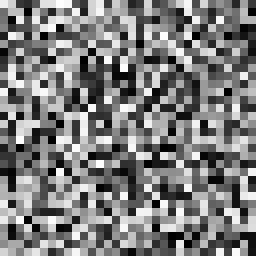
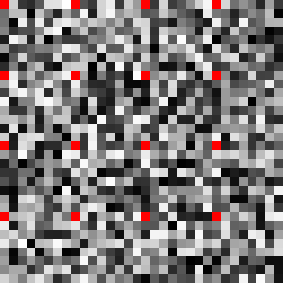
With all that in mind, our only work here is to generate a height map representing a terrain. Let’s start by randomly generating one of those. For each grid value (or pixel), we assign a random real number between 0 and 1. If you click on the dark box below, you will see both the generated height map and the corresponding terrain (please be patient if the 3D terrain generation freezes your browser for several seconds, sorry about that!).

Well, without surprise, this does not look really realistic. We obtain a grassy-looking terrain, far from anything we could find in real life. This terrain lacks two features. Firstly, it needs continuity. In a real landscape, we could not find such brisk variations. There is too much height difference between neighbor vertices; it’s too abrupt, not smooth enough.

Secondly, it lacks several levels of precision. Imagine for a moment that we solved the first issue by only giving random values to some pixels and using these pixels as guides to determine the height of the others by interpolation. Like when you pull a cloth up, your action is only applied to a specific point but every surrounding vertices rise too. Well, even with this workaround our terrain won’t be realistic enough because it will only be composed of flat and artificial slopes. When looking at a mountain from afar, you can merely observe the general outline. If you walk closer, some hills and valleys start to appear. When you’re on the mountain itself, you can see very tiny details, small holes, rocks. To give our terrain a natural feel, we need to capture variations both at the macroscopic and microscopic levels.

This is when value noise (not to be confused with Perlin noise) comes into play. The steps described below let us create a more natural-looking terrain from the random one we just generated:

1. Sample n regular subsets of pixels where each subset contains specific pixels which will guide the global relief.

2. Fill the gaps between the selected pixels with some kind of interpolation

3. Sum up each of these layers with appropriate weights to obtain the final height map

Sampling

Sampling the original random noise at different levels provides us with the several layers of precision needed. Each of these sampled maps is called an octave and is associated with a number i where octave i is the layer containing all pixels from the original height map which x-coordinate AND y-coordinate are multiple of 2ⁱ.

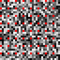
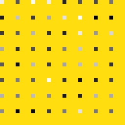
Let’s take the following 64*64 randomly generated height map as an example.

Note that octave 0 actually is the random noise as it contains every pixel since all coordinates are multiple of 2⁰ = 1.

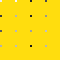
Let’s compute octave 1: only the pixels at valid coordinates (in red) are kept and the yellow color represents an absence of value.

For octave 2, there are less grid cells and of course they are larger. we remark that the sampled pixels form a grid.

We can continue with octave 3. The yellow space is growing and the gist of the next step will be to fill these empty zones.

Filling the gaps

For the moment, octave are mainly empty, apart from the sampled points. These points will serve as guides and we want the slopes between each pair of sampled points to be continuous (remember the cloth metaphor).

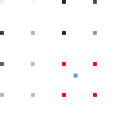
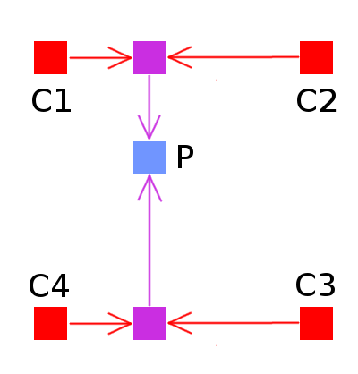
So we need to determine the values of absent pixels. Let’s say we want to compute the height of pixel P of a given octave. To do so, we simply find in which square P is and interpolate the heights of its corners with respect to the distance from P to each corner. in the following illustration, P is the blue pixel which height we want to compute and the corners of its square are red.

Several kinds of interpolation are available. The simplest is linear interpolation; efficient in terms of speed but the result can be a bit rough (check this page for more interpolation methods).

function linear(a, b, x) {
  return a + (b - a) * x;
}

a is the starting value, b the ending value and x a ratio. If x is 0 then the result is a. If x is 1 then the result is b. More generally, the higher x is, the closer the result is to b.

> linear(0, 10, 0.5)
5

> linear(1, 2, 0.1)
1.1

> linear(0, 100, 0.8)
80

You will note that the given functions only work in 1D. To obtain the value of P from the four corner of the square (C1, C2, C3, C4), we separately interpolate (C1 and C2) and (C3 and C4) using P abscissa as the x ratio which gives us the values of points respectively at the top and bottom lines of the square. Then we interpolate these two intermediate points using P ordinate as the ratio. This process is known as bilinear interpolation.

So what we have to do simply is to apply this method on every empty pixel of each octave. The result is a collection of continuous octaves bearing varying granularities. The following demo shows the third and fifth octaves based on the random noise generated earlier. The results appear rather smooth because I used cosine interpolation instead of the linear one which would have produced more pointy hills but the principle is absolutely identical.

Summing up

Let’s summarize. From a unique random noise, we created octaves by regularly sampling pixels and we filled the voids between these using interpolation. The last step is to merge the octaves into the final height map.

It’s rather straightforward to assume that the octave with the highest granularity is going to help define the global relief whereas the one with the smallest will only influe on small local details. The first intuition naturally is to average the heights of the pixel from each octave. In the following equation F_x,y is the height of the pixel at coordinates (x, y) in the final height map, O_i(x,y) is the height of the same pixel in the i-th octave :

The sum of all heights is normalized so that the final height value still lies within [0,1].

But this not precise enough, with this formula the terrain will only look like random noise. In order to make good use of our different layers of precision, the influence of each of them in the final result is weighted and obviously the higher the octave, the higher its influence will be. This phenomenom can be simulated by a new fixed quantity, the persistence P, a real number between 0 and 1 describing the increase of influence of the higher octaves.

With the weighting function W, the merge formula becomes:

Note that the normalization part has changed to accomodate the different weights applied.

Here is the JavaScript version of the merging process.

function valueNoise(x, y, k, source) {

   // Compute the height of pixel (x,y) in octaves 0 to k.
   var octaves = [source[x][y]];
   for(var i = 1; i <= k; ++i)
		octaves[i] = octave(x, y, i, source);

   // Reverse the order of the octaves so that the higher
   // is added first.
   octaves.reverse();

   // Start by adding the full height of the pixel from
   // the higher octave.
   var height = octaves[0];
   var weight = 1;
   var sumWeight = weight;

   // Describes the drop-off of influence with each layer.
   var persistence = 0.55;

   for(var i = 1; i <= k ; ++i) {

      // Decrease the influence of the current octave.
      weight = Math.pow(persistence, i);

      // Add the weighted height of the pixel to the
      // final height map.
      height += octaves[i] * weight;

      sumWeight += weight;
   }

   // Normalize the height.
   height /= sumAmplitude;

   return height;
}

Behold, our final terrain!